网站建设最好的公司排名潮州网络推广
目录
- 1. 说明
- 2. 猫狗大战
- 2.1 导入相关库
- 2.2 建立模型
- 2.3 模型编译
- 2.4 数据生成器
- 2.5 模型训练
- 2.6 模型保存
- 2.7 模型训练结果的可视化
- 3. 猫狗大战的CNN模型可视化结果图
- 4. 完整代码
- 5. 猫狗大战的迁移学习
1. 说明
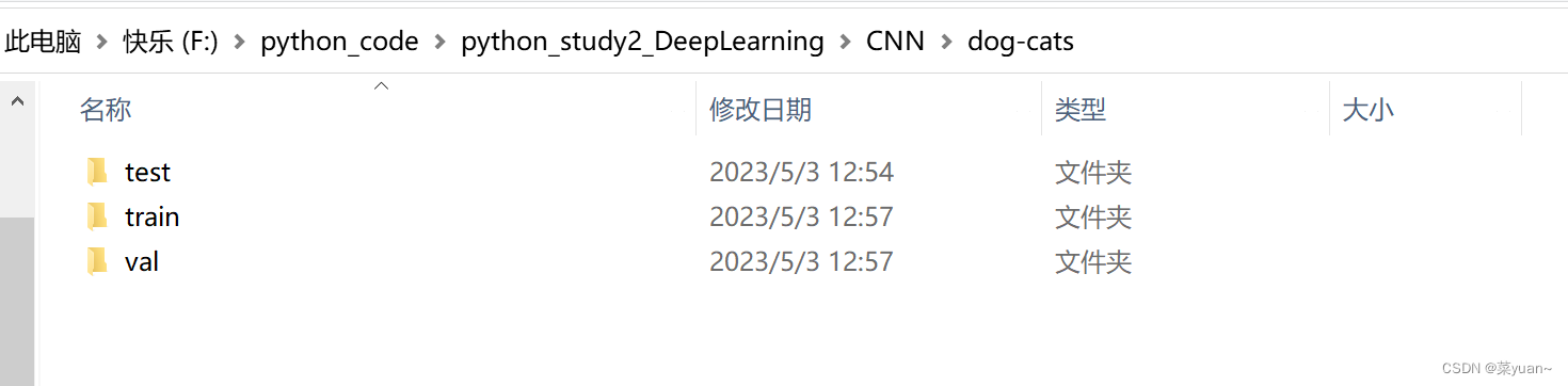
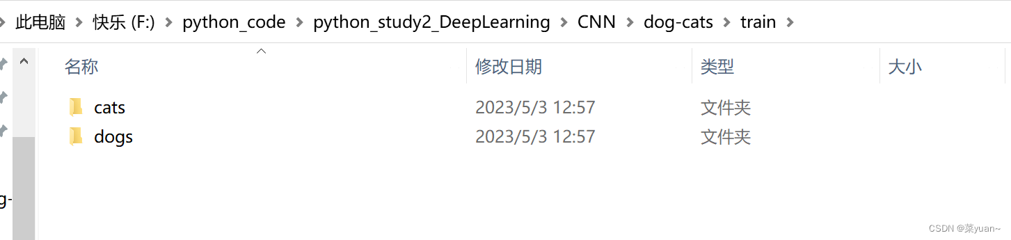
本篇文章是CNN的另外一个例子,猫狗大战,是自制数据集的例子。之前的例子都是python中库自带的,但是这次的例子是自己搜集数据集,如下图所示整理,数据集的链接会放在评论区。
2. 猫狗大战
2.1 导入相关库
以下第三方库是python专门用于深度学习的库
from keras.models import Sequential
from keras.layers import Dense, Conv2D, Flatten, Dropout, BatchNormalization
from keras.optimizers import RMSprop, Adam
from keras.preprocessing.image import ImageDataGenerator
import sys, os  # 目录结构
from keras.layers import MaxPool2D
import matplotlib.pyplot as plt
import pandas
from keras.callbacks import EarlyStopping, ReduceLROnPlateau
2.2 建立模型
这是采用另外一种书写方式建立模型。
构建了三层卷积层,三层池化层,然后是展平层(将二维特征图拉直输入给全连接层),然后是三层全连接层,并且加入了dropout层。
"1.模型建立"
# 1.卷积层,输入图片大小(150, 150, 3), 卷积核个数16,卷积核大小(5, 5), 激活函数'relu'
conv_layer1 = Conv2D(input_shape=(150, 150, 3), filters=16, kernel_size=(5, 5), activation='relu')
# 2.最大池化层,池化层大小(2, 2), 步长为2
max_pool1 = MaxPool2D(pool_size=(2, 2), strides=2)
# 3.卷积层,卷积核个数32,卷积核大小(5, 5), 激活函数'relu'
conv_layer2 = Conv2D(filters=32, kernel_size=(5, 5), activation='relu')
# 4.最大池化层,池化层大小(2, 2), 步长为2
max_pool2 = MaxPool2D(pool_size=(2, 2), strides=2)
# 5.卷积层,卷积核个数64,卷积核大小(5, 5), 激活函数'relu'
conv_layer3 = Conv2D(filters=64, kernel_size=(5, 5), activation='relu')
# 6.最大池化层,池化层大小(2, 2), 步长为2
max_pool3 = MaxPool2D(pool_size=(2, 2), strides=2)
# 7.卷积层,卷积核个数128,卷积核大小(5, 5), 激活函数'relu'
conv_layer4 = Conv2D(filters=128, kernel_size=(5, 5), activation='relu')
# 8.最大池化层,池化层大小(2, 2), 步长为2
max_pool4 = MaxPool2D(pool_size=(2, 2), strides=2)
# 9.展平层
flatten_layer = Flatten()
# 10.Dropout层, Dropout(0.2)
third_dropout = Dropout(0.2)
# 11.全连接层/隐藏层1,240个节点, 激活函数'relu'
hidden_layer1 = Dense(240, activation='relu')
# 12.全连接层/隐藏层2,84个节点, 激活函数'relu'
hidden_layer3 = Dense(84, activation='relu')
# 13.Dropout层, Dropout(0.2)
fif_dropout = Dropout(0.5)
# 14.输出层,输出节点个数1, 激活函数'sigmoid'
output_layer = Dense(1, activation='sigmoid')
model = Sequential([conv_layer1, max_pool1, conv_layer2, max_pool2,conv_layer3, max_pool3, conv_layer4, max_pool4,flatten_layer, third_dropout, hidden_layer1,hidden_layer3, fif_dropout, output_layer])
2.3 模型编译
模型的优化器是Adam,学习率是0.01,
损失函数是binary_crossentropy,二分类交叉熵,
性能指标是正确率accuracy,
另外还加入了回调机制。
回调机制简单理解为训练集的准确率持续上升,而验证集准确率基本不变,此时已经出现过拟合,应该调制学习率,让验证集的准确率也上升。
"2.模型编译"
# 模型编译,2分类:binary_crossentropy
model.compile(optimizer=Adam(lr=0.0001),  # 优化器选择Adam,初始学习率设置为0.0001loss='binary_crossentropy',  # 代价函数选择 binary_crossentropymetrics=['accuracy'])  # 设置指标为准确率
model.summary()  # 模型统计# 回调机制 动态调整学习率
reduce = ReduceLROnPlateau(monitor='val_accuracy',  # 设置监测的值为val_accuracypatience=2,  # 设置耐心容忍次数为2verbose=1,  #factor=0.5,  # 缩放学习率的值为0.5,学习率将以lr = lr*factor的形式被减少min_lr=0.000001  # 学习率最小值0.000001)   # 监控val_accuracy增加趋势
2.4 数据生成器
加载自制数据集
利用数据生成器对数据进行数据加强,即每次训练时输入的图片会是原图片的翻转,平移,旋转,缩放,这样是为了降低过拟合的影响。
然后通过迭代器进行数据加载,目标图像大小统一尺寸1501503,设置每次加载到训练网络的图像数目,设置而分类模型(默认one-hot编码),并且数据打乱。
"3.数据生成器"
# 生成器对象1:  归一化
gen = ImageDataGenerator(rescale=1 / 255.0)
# 生成器对象2:  归一化 + 数据加强
gen1 = ImageDataGenerator(rescale=1 / 255.0,rotation_range=5,  # 图片随机旋转的角度5度width_shift_range=0.1,height_shift_range=0.1,  # 水平和竖直方向随机移动0.1shear_range=0.1,  # 剪切变换的程度0.1zoom_range=0.1,  # 随机放大的程度0.1fill_mode='nearest')  # 当需要进行像素填充时选择最近的像素进行填充
# 拼接训练和验证的两个路径
train_path = os.path.join(sys.path[0], 'dog-cats', 'train')
val_path = os.path.join(sys.path[0], 'dog-cats', 'val')
print('训练数据路径: ', train_path)
print('验证数据路径: ', val_path)
# 训练和验证的两个迭代器
train_iter = gen1.flow_from_directory(train_path,  # 训练train目录路径target_size=(150, 150),  # 目标图像大小统一尺寸150batch_size=8,  # 设置每次加载到内存的图像大小class_mode='binary',  # 设置分类模型(默认one-hot编码)shuffle=True)  # 是否打乱
val_iter = gen.flow_from_directory(val_path,  # 测试val目录路径target_size=(150, 150),  # 目标图像大小统一尺寸150batch_size=8,  # 设置每次加载到内存的图像大小class_mode='binary',  # 设置分类模型(默认one-hot编码)shuffle=True)  # 是否打乱
2.5 模型训练
模型训练的次数是20,每1次循环进行测试
"4.模型训练"
# 模型的训练, model.fit
result = model.fit(train_iter,  # 设置训练数据的迭代器epochs=20,  # 循环次数20次validation_data=val_iter,  # 验证数据的迭代器callbacks=[reduce],  # 回调机制设置为reduceverbose=1)
2.6 模型保存
以.h5文件格式保存模型
"5.模型保存"
# 保存训练好的模型
model.save('my_cnn_cat_dog.h5')
2.7 模型训练结果的可视化
对模型的训练结果进行可视化,可视化的结果用曲线图的形式展现
"6.模型训练时的可视化"
# 显示训练集和验证集的acc和loss曲线
acc = result.history['accuracy']  # 获取模型训练中的accuracy
val_acc = result.history['val_accuracy']  # 获取模型训练中的val_accuracy
loss = result.history['loss']  # 获取模型训练中的loss
val_loss = result.history['val_loss']  # 获取模型训练中的val_loss
# 绘值acc曲线
plt.figure(1)
plt.plot(acc, label='Training Accuracy')
plt.plot(val_acc, label='Validation Accuracy')
plt.title('Training and Validation Accuracy')
plt.legend()
plt.savefig('cat_dog_acc.png', dpi=600)
# 绘制loss曲线
plt.figure(2)
plt.plot(loss, label='Training Loss')
plt.plot(val_loss, label='Validation Loss')
plt.title('Training and Validation Loss')
plt.legend()
plt.savefig('cat_dog_loss.png', dpi=600)
plt.show()  # 将结果显示出来
3. 猫狗大战的CNN模型可视化结果图
Epoch 1/20
250/250 [==============================] - 59s 231ms/step - loss: 0.6940 - accuracy: 0.4925 - val_loss: 0.6899 - val_accuracy: 0.5050 - lr: 1.0000e-04
Epoch 2/20
250/250 [==============================] - 55s 219ms/step - loss: 0.6891 - accuracy: 0.5125 - val_loss: 0.6787 - val_accuracy: 0.5880 - lr: 1.0000e-04
Epoch 3/20
250/250 [==============================] - 54s 216ms/step - loss: 0.6791 - accuracy: 0.5840 - val_loss: 0.6655 - val_accuracy: 0.6080 - lr: 1.0000e-04
Epoch 4/20
250/250 [==============================] - 60s 238ms/step - loss: 0.6628 - accuracy: 0.6040 - val_loss: 0.6501 - val_accuracy: 0.6300 - lr: 1.0000e-04
Epoch 5/20
250/250 [==============================] - 57s 226ms/step - loss: 0.6480 - accuracy: 0.6400 - val_loss: 0.6281 - val_accuracy: 0.6590 - lr: 1.0000e-04
Epoch 6/20
250/250 [==============================] - 67s 268ms/step - loss: 0.6275 - accuracy: 0.6565 - val_loss: 0.6160 - val_accuracy: 0.6690 - lr: 1.0000e-04
Epoch 7/20
250/250 [==============================] - 62s 247ms/step - loss: 0.6252 - accuracy: 0.6570 - val_loss: 0.6026 - val_accuracy: 0.6790 - lr: 1.0000e-04
Epoch 8/20
250/250 [==============================] - 63s 251ms/step - loss: 0.5915 - accuracy: 0.6770 - val_loss: 0.5770 - val_accuracy: 0.6960 - lr: 1.0000e-04
Epoch 9/20
250/250 [==============================] - 57s 228ms/step - loss: 0.5778 - accuracy: 0.6930 - val_loss: 0.5769 - val_accuracy: 0.6880 - lr: 1.0000e-04
Epoch 10/20
250/250 [==============================] - 55s 219ms/step - loss: 0.5532 - accuracy: 0.7085 - val_loss: 0.5601 - val_accuracy: 0.6970 - lr: 1.0000e-04
Epoch 11/20
250/250 [==============================] - 55s 221ms/step - loss: 0.5408 - accuracy: 0.7370 - val_loss: 0.6002 - val_accuracy: 0.6810 - lr: 1.0000e-04
Epoch 12/20
250/250 [==============================] - ETA: 0s - loss: 0.5285 - accuracy: 0.7350
Epoch 12: ReduceLROnPlateau reducing learning rate to 4.999999873689376e-05.
250/250 [==============================] - 56s 226ms/step - loss: 0.5285 - accuracy: 0.7350 - val_loss: 0.5735 - val_accuracy: 0.6960 - lr: 1.0000e-04
Epoch 13/20
250/250 [==============================] - 70s 280ms/step - loss: 0.4969 - accuracy: 0.7595 - val_loss: 0.5212 - val_accuracy: 0.7410 - lr: 5.0000e-05
Epoch 14/20
250/250 [==============================] - 73s 292ms/step - loss: 0.4776 - accuracy: 0.7740 - val_loss: 0.5146 - val_accuracy: 0.7470 - lr: 5.0000e-05
Epoch 15/20
250/250 [==============================] - 71s 285ms/step - loss: 0.4605 - accuracy: 0.7930 - val_loss: 0.5180 - val_accuracy: 0.7530 - lr: 5.0000e-05
Epoch 16/20
250/250 [==============================] - 74s 298ms/step - loss: 0.4619 - accuracy: 0.7825 - val_loss: 0.5100 - val_accuracy: 0.7510 - lr: 5.0000e-05
Epoch 17/20
250/250 [==============================] - 72s 289ms/step - loss: 0.4558 - accuracy: 0.7885 - val_loss: 0.4991 - val_accuracy: 0.7630 - lr: 5.0000e-05
Epoch 18/20
250/250 [==============================] - 75s 300ms/step - loss: 0.4498 - accuracy: 0.7900 - val_loss: 0.4966 - val_accuracy: 0.7580 - lr: 5.0000e-05
Epoch 19/20
250/250 [==============================] - 61s 243ms/step - loss: 0.4269 - accuracy: 0.8060 - val_loss: 0.5000 - val_accuracy: 0.7690 - lr: 5.0000e-05
Epoch 20/20
250/250 [==============================] - 56s 224ms/step - loss: 0.4202 - accuracy: 0.8090 - val_loss: 0.4845 - val_accuracy: 0.7700 - lr: 5.0000e-05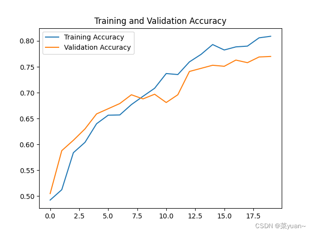
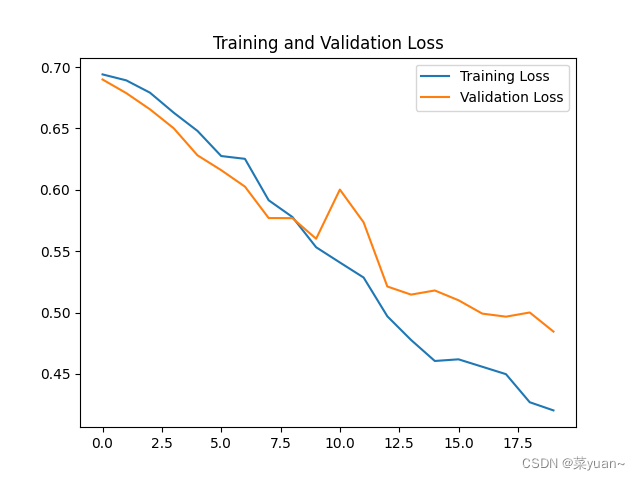
从以上结果可知,模型的准确率达到了77%。可以发现并不是很高,因此采用下面的迁移学习。
4. 完整代码
from keras.models import Sequential
from keras.layers import Dense, Conv2D, Flatten, Dropout, BatchNormalization
from keras.optimizers import RMSprop, Adam
from keras.preprocessing.image import ImageDataGenerator
import sys, os  # 目录结构
from keras.layers import MaxPool2D
import matplotlib.pyplot as plt
import pandas
from keras.callbacks import EarlyStopping, ReduceLROnPlateau"1.模型建立"
# 1.卷积层,输入图片大小(150, 150, 3), 卷积核个数16,卷积核大小(5, 5), 激活函数'relu'
conv_layer1 = Conv2D(input_shape=(150, 150, 3), filters=16, kernel_size=(5, 5), activation='relu')
# 2.最大池化层,池化层大小(2, 2), 步长为2
max_pool1 = MaxPool2D(pool_size=(2, 2), strides=2)
# 3.卷积层,卷积核个数32,卷积核大小(5, 5), 激活函数'relu'
conv_layer2 = Conv2D(filters=32, kernel_size=(5, 5), activation='relu')
# 4.最大池化层,池化层大小(2, 2), 步长为2
max_pool2 = MaxPool2D(pool_size=(2, 2), strides=2)
# 5.卷积层,卷积核个数64,卷积核大小(5, 5), 激活函数'relu'
conv_layer3 = Conv2D(filters=64, kernel_size=(5, 5), activation='relu')
# 6.最大池化层,池化层大小(2, 2), 步长为2
max_pool3 = MaxPool2D(pool_size=(2, 2), strides=2)
# 7.卷积层,卷积核个数128,卷积核大小(5, 5), 激活函数'relu'
conv_layer4 = Conv2D(filters=128, kernel_size=(5, 5), activation='relu')
# 8.最大池化层,池化层大小(2, 2), 步长为2
max_pool4 = MaxPool2D(pool_size=(2, 2), strides=2)
# 9.展平层
flatten_layer = Flatten()
# 10.Dropout层, Dropout(0.2)
third_dropout = Dropout(0.2)
# 11.全连接层/隐藏层1,240个节点, 激活函数'relu'
hidden_layer1 = Dense(240, activation='relu')
# 12.全连接层/隐藏层2,84个节点, 激活函数'relu'
hidden_layer3 = Dense(84, activation='relu')
# 13.Dropout层, Dropout(0.2)
fif_dropout = Dropout(0.5)
# 14.输出层,输出节点个数1, 激活函数'sigmoid'
output_layer = Dense(1, activation='sigmoid')
model = Sequential([conv_layer1, max_pool1, conv_layer2, max_pool2,conv_layer3, max_pool3, conv_layer4, max_pool4,flatten_layer, third_dropout, hidden_layer1,hidden_layer3, fif_dropout, output_layer])
"2.模型编译"
# 模型编译,2分类:binary_crossentropy
model.compile(optimizer=Adam(lr=0.0001),  # 优化器选择Adam,初始学习率设置为0.0001loss='binary_crossentropy',  # 代价函数选择 binary_crossentropymetrics=['accuracy'])  # 设置指标为准确率
model.summary()  # 模型统计# 回调机制 动态调整学习率
reduce = ReduceLROnPlateau(monitor='val_accuracy',  # 设置监测的值为val_accuracypatience=2,  # 设置耐心容忍次数为2verbose=1,  #factor=0.5,  # 缩放学习率的值为0.5,学习率将以lr = lr*factor的形式被减少min_lr=0.000001  # 学习率最小值0.000001)   # 监控val_accuracy增加趋势
"3.数据生成器"
# 生成器对象1:  归一化
gen = ImageDataGenerator(rescale=1 / 255.0)
# 生成器对象2:  归一化 + 数据加强
gen1 = ImageDataGenerator(rescale=1 / 255.0,rotation_range=5,  # 图片随机旋转的角度5度width_shift_range=0.1,height_shift_range=0.1,  # 水平和竖直方向随机移动0.1shear_range=0.1,  # 剪切变换的程度0.1zoom_range=0.1,  # 随机放大的程度0.1fill_mode='nearest')  # 当需要进行像素填充时选择最近的像素进行填充
# 拼接训练和验证的两个路径
train_path = os.path.join(sys.path[0], 'dog-cats', 'train')
val_path = os.path.join(sys.path[0], 'dog-cats', 'val')
print('训练数据路径: ', train_path)
print('验证数据路径: ', val_path)
# 训练和验证的两个迭代器
train_iter = gen1.flow_from_directory(train_path,  # 训练train目录路径target_size=(150, 150),  # 目标图像大小统一尺寸150batch_size=8,  # 设置每次加载到内存的图像大小class_mode='binary',  # 设置分类模型(默认one-hot编码)shuffle=True)  # 是否打乱
val_iter = gen.flow_from_directory(val_path,  # 测试val目录路径target_size=(150, 150),  # 目标图像大小统一尺寸150batch_size=8,  # 设置每次加载到内存的图像大小class_mode='binary',  # 设置分类模型(默认one-hot编码)shuffle=True)  # 是否打乱
"4.模型训练"
# 模型的训练, model.fit
result = model.fit(train_iter,  # 设置训练数据的迭代器epochs=20,  # 循环次数20次validation_data=val_iter,  # 验证数据的迭代器callbacks=[reduce],  # 回调机制设置为reduceverbose=1)"5.模型保存"
# 保存训练好的模型
model.save('my_cnn_cat_dog.h5')"6.模型训练时的可视化"
# 显示训练集和验证集的acc和loss曲线
acc = result.history['accuracy']  # 获取模型训练中的accuracy
val_acc = result.history['val_accuracy']  # 获取模型训练中的val_accuracy
loss = result.history['loss']  # 获取模型训练中的loss
val_loss = result.history['val_loss']  # 获取模型训练中的val_loss
# 绘值acc曲线
plt.figure(1)
plt.plot(acc, label='Training Accuracy')
plt.plot(val_acc, label='Validation Accuracy')
plt.title('Training and Validation Accuracy')
plt.legend()
plt.savefig('cat_dog_acc.png', dpi=600)
# 绘制loss曲线
plt.figure(2)
plt.plot(loss, label='Training Loss')
plt.plot(val_loss, label='Validation Loss')
plt.title('Training and Validation Loss')
plt.legend()
plt.savefig('cat_dog_loss.png', dpi=600)
plt.show()  # 将结果显示出来
5. 猫狗大战的迁移学习
迁移学习简单来说就是将别人已经训练好的模型拿来自己用。
from keras.applications import DenseNet121
from keras.models import Sequential
from keras.layers import Dense, Conv2D, Flatten, Dropout, BatchNormalization
from keras.optimizers import RMSprop, Adam
from keras.preprocessing.image import ImageDataGenerator
import sys, os  # 目录结构
from keras.layers import MaxPool2D
import matplotlib.pyplot as plt
import pandas
from keras.callbacks import EarlyStopping, ReduceLROnPlateau"1.模型建立"
# 加载DenseNet网络模型,并去掉最后一层全连接层,最后一个池化层设置为max pooling
net = DenseNet121(weights='imagenet', include_top=False, pooling='max')
# 设计为不参与优化,即MobileNet这部分参数固定不动
net.trainable = False
newnet = Sequential([net,  # 去掉最后一层的DenseNet121Dense(1024, activation='relu'),  # 追加全连接层BatchNormalization(),  # 追加BN层Dropout(rate=0.5),  # 追加Dropout层,防止过拟合Dense(1,activation='sigmoid') # 根据宝可梦数据的任务,设置最后一层输出节点数为5
])
newnet.build(input_shape=(None, 150, 150, 3))"2.模型编译"
newnet.compile(optimizer=Adam(lr=0.0001), loss="binary_crossentropy", metrics=["accuracy"])
newnet.summary()# 回调机制 动态调整学习率
reduce = ReduceLROnPlateau(monitor='val_accuracy',  # 设置监测的值为val_accuracypatience=2,  # 设置耐心容忍次数为2verbose=1,  #factor=0.5,  # 缩放学习率的值为0.5,学习率将以lr = lr*factor的形式被减少min_lr=0.000001  # 学习率最小值0.000001)   # 监控val_accuracy增加趋势"3.数据生成器"
# 生成器对象1:  归一化
gen = ImageDataGenerator(rescale=1 / 255.0)
# 生成器对象2:  归一化 + 数据加强
gen1 = ImageDataGenerator(rescale=1 / 255.0,rotation_range=5,  # 图片随机旋转的角度5度width_shift_range=0.1,height_shift_range=0.1,  # 水平和竖直方向随机移动0.1shear_range=0.1,  # 剪切变换的程度0.1zoom_range=0.1,  # 随机放大的程度0.1fill_mode='nearest')  # 当需要进行像素填充时选择最近的像素进行填充
# 拼接训练和验证的两个路径
train_path = os.path.join(sys.path[0], 'dog-cats', 'train')
val_path = os.path.join(sys.path[0], 'dog-cats', 'val')
print('训练数据路径: ', train_path)
print('验证数据路径: ', val_path)
# 训练和验证的两个迭代器
train_iter = gen1.flow_from_directory(train_path,  # 训练train目录路径target_size=(150, 150),  # 目标图像大小统一尺寸150batch_size=10,  # 设置每次加载到内存的图像大小class_mode='binary',  # 设置分类模型(默认one-hot编码)shuffle=True)  # 是否打乱
val_iter = gen.flow_from_directory(val_path,  # 测试val目录路径target_size=(150, 150),  # 目标图像大小统一尺寸150batch_size=10,  # 设置每次加载到内存的图像大小class_mode='binary',  # 设置分类模型(默认one-hot编码)shuffle=True)  # 是否打乱
"4.模型训练"
# 模型的训练, newnet.fit
result = newnet.fit(train_iter,  # 设置训练数据的迭代器epochs=20,  # 循环次数20次validation_data=val_iter,  # 验证数据的迭代器callbacks=[reduce],  # 回调机制设置为reduceverbose=1)"5.模型保存"
# 保存训练好的模型
newnet.save('my_cnn_cat_dog_3.h5')"6.模型训练时的可视化"
# 显示训练集和验证集的acc和loss曲线
acc = result.history['accuracy']  # 获取模型训练中的accuracy
val_acc = result.history['val_accuracy']  # 获取模型训练中的val_accuracy
loss = result.history['loss']  # 获取模型训练中的loss
val_loss = result.history['val_loss']  # 获取模型训练中的val_loss
# 绘值acc曲线
plt.figure(1)
plt.plot(acc, label='Training Accuracy')
plt.plot(val_acc, label='Validation Accuracy')
plt.title('Training and Validation Accuracy')
plt.legend()
plt.savefig('cat_dog_acc_3.png', dpi=600)
# 绘制loss曲线
plt.figure(2)
plt.plot(loss, label='Training Loss')
plt.plot(val_loss, label='Validation Loss')
plt.title('Training and Validation Loss')
plt.legend()
plt.savefig('cat_dog_loss_3.png', dpi=600)
plt.show()  # 将结果显示出来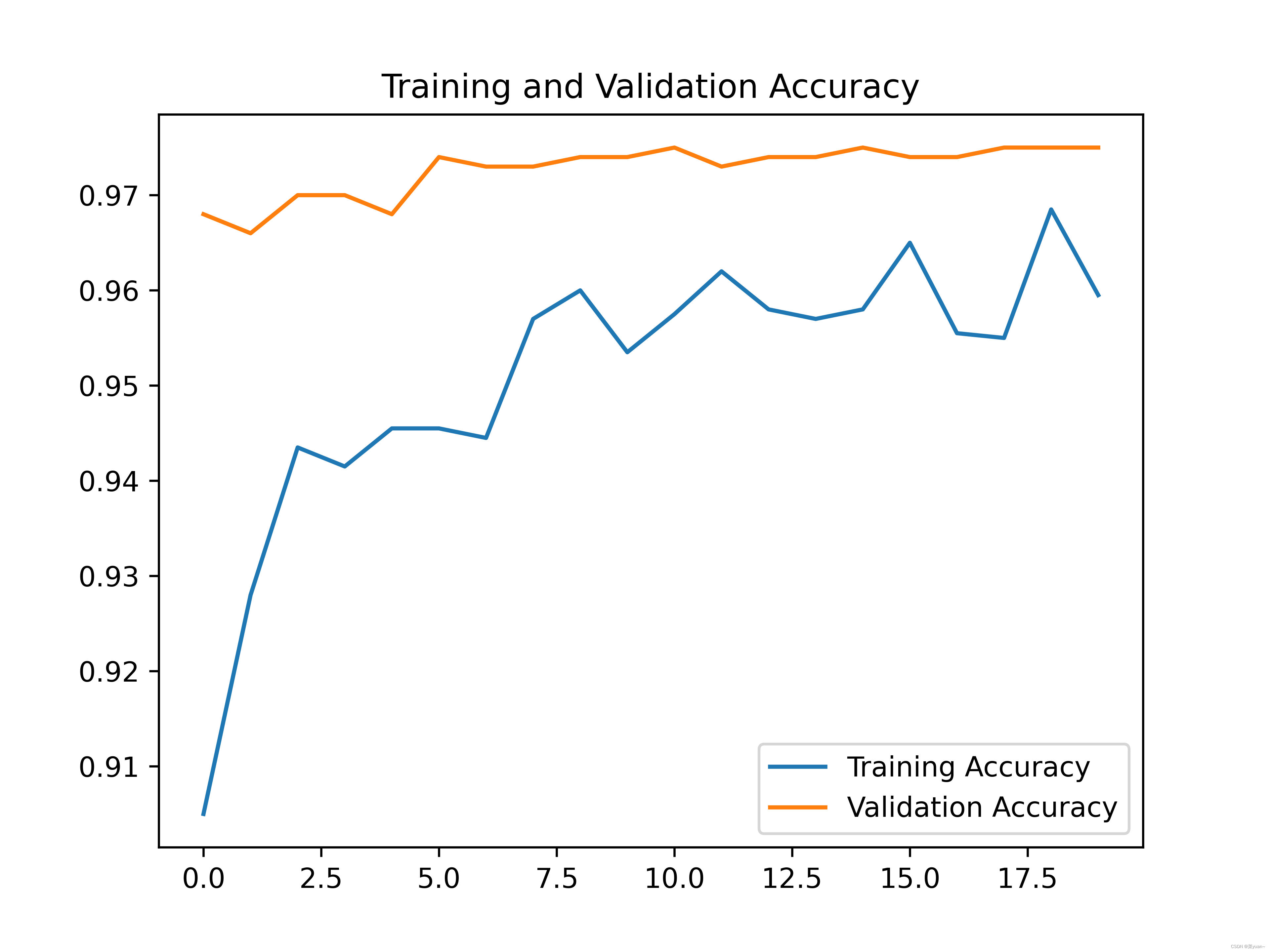
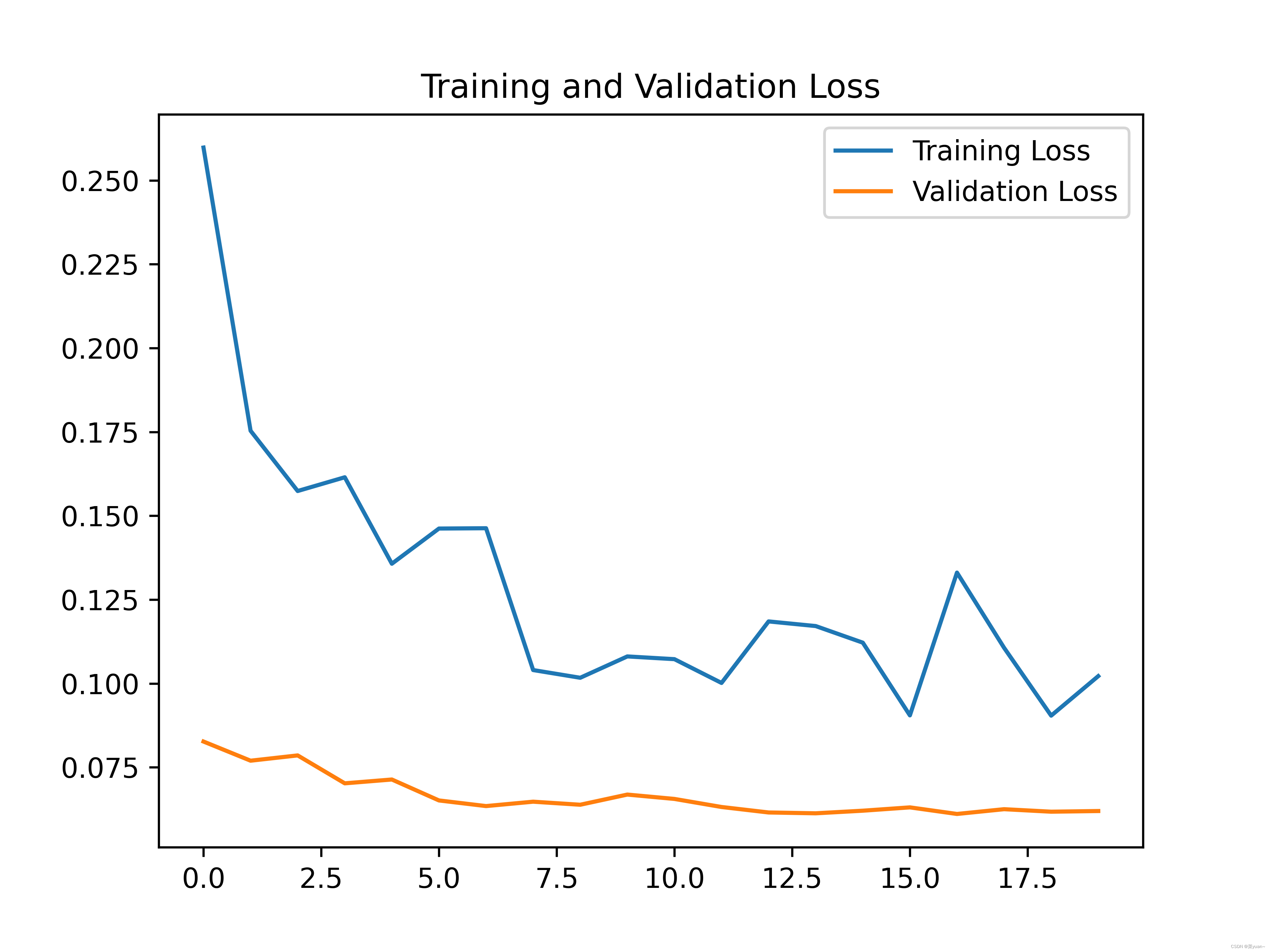
可以发现,通过迁移学习之后的模型准确率达到了96%。